\(\newcommand{\Z}{\mathbb{Z}} \newcommand{\reals}{\mathbb{R}} \newcommand{\real}[1]{\mathbb{R}^{#1}} \newcommand{\fe}[2]{#1\mathopen{}\left(#2\right)\mathclose{}} \newcommand{\cinterval}[2]{\left[#1,#2\right]} \newcommand{\ointerval}[2]{\left(#1,#2\right)} \newcommand{\cointerval}[2]{\left[\left.#1,#2\right)\right.} \newcommand{\ocinterval}[2]{\left(\left.#1,#2\right]\right.} \newcommand{\point}[2]{\left(#1,#2\right)} \newcommand{\fd}[1]{#1'} \newcommand{\sd}[1]{#1''} \newcommand{\td}[1]{#1'''} \newcommand{\lz}[2]{\frac{d#1}{d#2}} \newcommand{\lzn}[3]{\frac{d^{#1}#2}{d#3^{#1}}} \newcommand{\lzo}[1]{\frac{d}{d#1}} \newcommand{\lzoo}[2]{{\frac{d}{d#1}}{\left(#2\right)}} \newcommand{\lzon}[2]{\frac{d^{#1}}{d#2^{#1}}} \newcommand{\lzoa}[3]{\left.{\frac{d#1}{d#2}}\right|_{#3}} \newcommand{\abs}[1]{\left|#1\right|} \newcommand{\sech}{\operatorname{sech}} \newcommand{\csch}{\operatorname{csch}} \newcommand \dd[1] { \,\textrm d{#1} } \newcommand \de[2] { \frac{\mathrm d{#1}}{\mathrm d{#2}} } \newcommand \intl[4]{ \int\limits_{#1}^{#2}{#3}\dd{#4} } \newcommand\at[2]{\left.#1\right|_{#2}} \newcommand{\lt}{ < } \newcommand{\gt}{ > } \newcommand{\amp}{ & } \)

Section1.1SageMath Online

Probably the easiest way to familiarise yourself with SageMath is to use the Sage Math Cloud Server. From the main SageMath page select the Sage Online link. You will have to set up an account but these are free for basic usage.

Once you have set up an account you can then create a project and a SageMath Worksheet. There are full instructions here Logging On.
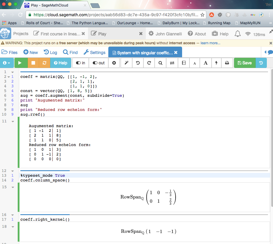
Figure1.1.1A Typical Sage Cloud Session

Notice the line %typeset_mode True just before the coeff.column_space() command. As you can see from the output below this line, this has the effect of displaying results in a much prettier (typeset) format.