Section4.1First Order Differential Equations¶ permalink
Subsection4.1.1First Example
For this first example, we'll look at a simple problem so that we can concentrate on the SageMath commands without having to deal with the mathematical details.
\begin{equation}\frac{dy}{dx} + y(x) - 3 = 0\label{men-8}\tag{4.1.1}\end{equation}\begin{equation}y(0) = 1\label{men-9}\tag{4.1.2}\end{equation}Subsubsection4.1.1.1The General Solution
First define \(y\) as a function of \(x\)
Next define our DE. Notice the '==' rather than the '=' when setting the RHS to zero. We are defining a Sage variable '\(de\)' to hold the differential equation. The first '=' is to set the variable \(de\) equal to our DE.
The derivative(y,x) is a Sage method that is passed a function, in this case \(y\). Of course, this has been defined above as \(y(x)\). The derivative() method also takes one or more additional arguments for the equation variable, in this case \(x\).
This is a good point to talk about the Sage help facility.
Try the following:
This is a typical Docstring output detailing the signature (the required arguments) and details on how to use the method.
Notice that an alias for this method id diff. In other words an alias for derivative(y,x) would be diff(y,x).
Now for the general solution. For this we use the desolve() method - differential equation solve. Try using 'desolve?' to list the built in documentation.
This is the general solution as can be seen by the \(_C\) constant.
Let us now do two things: store the solution into a variable, and display the solution in a prettier format:
\begin{equation}{\left(C + 3 \, e^{x}\right)} e^{\left(-x\right)}\label{men-10}\tag{4.1.3}\end{equation}
Subsubsection4.1.1.2Initial Conditions
The initial condition for this equation is \(y(0) = 1\). That is, at \(x = 0, y = 1\).
From the Docstring for desolve() you can see :
- "ics" - (optional) the initial or boundary conditions
- for a first-order equation, specify the initial "x" and "y"
So let us try it. Notice the [0,1] for the [x,y] initial conditions.
\begin{equation}{\left(3 \, e^{x} - 2\right)} e^{\left(-x\right)}\label{men-11}\tag{4.1.4}\end{equation}
Here we have again stored the solution to a variable sol_initial_con and used show() to pretty=print the output.
Subsubsection4.1.1.3Plotting the Solution
Have a look at the Docstring for method plot() (plot?).
From this you can see that how to graph from \(x=0..5\) and set the minimum y using \(ymin\):
Spend some time studying the other options.
Subsubsection4.1.1.4Numerical Solution
In practice most DE ar not solvable analytically and we have to resort to numerical methods.
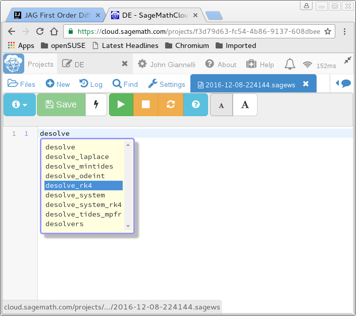
This is a good point to talk about the tab key and auto-completion.
Tab completion will not work in Sage Cells (what yo are using in this document) but only from a Sage Math Online sessions. 1.1
To illustrate, from an online workbook type desolve and press the tab key. All of the methods and actions that are possible to complete the method are displayed in a dop-down list. See the diagram below.

From the dropdown select the desolve_rk4 method. If required, now type '?' to display a description of this method.
These two solutions can be plotted together. As can be expected the \(+\) operator acting on two plots will display them together.
Subsubsection4.1.1.5Plotting the Vector Field
Let us re-write our original equation as:
\begin{equation}\frac{dy}{dx} = 3 - y(x)\label{men-12}\tag{4.1.5}\end{equation}There is a nice function plot_slope_field() that can be used to plot this equation over a range of \(x\) and \(y\).
Previously we defined \(y\) as a function. Here we have to redefine it as a variable.
If you plot this together with exact plot from above you can see that slope plot gives us a view of all the whole equation and not just a particular solution for a single set of initial conditions.
Subsection4.1.2Second Example
This second example models the relationship between a continuous waveform and a dependent system. The differential equation looks like this:
\begin{equation}y(t) + rc\frac{dy}{dt}(t) = sin(\omega t)\label{men-13}\tag{4.1.6}\end{equation}For this equation there is no initial value setting because the system being modeled is continuous. This equation models natural systems that have a driving sinusoidal waveform. Here is the process for solving it:
\begin{equation}{\left(C - \frac{{\left(\omega \cos\left(\omega t\right) - \frac{\sin\left(\omega t\right)}{c r}\right)} e^{\left(\frac{t}{c r}\right)}}{{\left(\omega^{2} + \frac{1}{c^{2} r^{2}}\right)} c r}\right)} e^{\left(-\frac{t}{c r}\right)} \label{men-14}\tag{4.1.7}\end{equation}
Although this is correct it is not in the canonical format that is more recognizable. This class of DE is actually rather difficult to solve because initial values are assumed to exist, and it's difficult to specify the equation without any implicit or explicit initial values.
First, when the desolve() function does not get an explicit initial value specification as in this case, Sage automatically assigns a variable to represent it. In the result shown the initial value variable is \( c\). The \(c\) variable assigned by desolve() is key to creating the desired equation.
Second, notice the appearance of the \(e^{\left(\frac{t}{c r}\right)}\) and \(e^{\left(-\frac{t}{c r}\right)} \) terms in the result. These are present because the DE solver wrongly assumes that an initial value is present or needed. The secret to putting this equation into the desired form is to remove these exponential terms. What you need to do is set the constant C ( _C in the raw Sage response) to zero:
\begin{equation}-\frac{c \omega r \cos\left(\omega t\right) - \sin\left(\omega t\right)}{c^{2} \omega^{2} r^{2} + 1} \label{men-15}\tag{4.1.8}\end{equation}
