\(\newcommand{\Z}{\mathbb{Z}} \newcommand{\reals}{\mathbb{R}} \newcommand{\real}[1]{\mathbb{R}^{#1}} \newcommand{\fe}[2]{#1\mathopen{}\left(#2\right)\mathclose{}} \newcommand{\cinterval}[2]{\left[#1,#2\right]} \newcommand{\ointerval}[2]{\left(#1,#2\right)} \newcommand{\cointerval}[2]{\left[\left.#1,#2\right)\right.} \newcommand{\ocinterval}[2]{\left(\left.#1,#2\right]\right.} \newcommand{\point}[2]{\left(#1,#2\right)} \newcommand{\fd}[1]{#1'} \newcommand{\sd}[1]{#1''} \newcommand{\td}[1]{#1'''} \newcommand{\lz}[2]{\frac{d#1}{d#2}} \newcommand{\lzn}[3]{\frac{d^{#1}#2}{d#3^{#1}}} \newcommand{\lzo}[1]{\frac{d}{d#1}} \newcommand{\lzoo}[2]{{\frac{d}{d#1}}{\left(#2\right)}} \newcommand{\lzon}[2]{\frac{d^{#1}}{d#2^{#1}}} \newcommand{\lzoa}[3]{\left.{\frac{d#1}{d#2}}\right|_{#3}} \newcommand{\abs}[1]{\left|#1\right|} \newcommand{\sech}{\operatorname{sech}} \newcommand{\csch}{\operatorname{csch}} \newcommand \dd[1] { \,\textrm d{#1} } \newcommand \de[2] { \frac{\mathrm d{#1}}{\mathrm d{#2}} } \newcommand \intl[4]{ \int\limits_{#1}^{#2}{#3}\dd{#4} } \newcommand\at[2]{\left.#1\right|_{#2}} \newcommand{\lt}{ < } \newcommand{\gt}{ > } \newcommand{\amp}{ & } \)

Section3.1Calculating Limits

The concept of the limit is often used to define the integral and the derivative of functions.

Here is an easy example to demonstrate Sage syntax for limits:

The following examples are taken from Essential Calculus - James Stewart [3.10.1].

See also the Sage Tutorial on Limits [3.10.2].

The examples here (and some more can all been found in this (public) Cloud SageMath Worksheet

Example 2, page 26

Plotting this function will give us a better picture of what is happening:
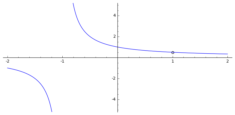
Figure3.1.1Example 2, page 26

Stewart : Section 1.3, Exercise 12, page 33

From a plot or simplification of the equation you can visually see that there is an explosion at \(-1\).

Note that we have used an exclude list (square brackets is a list) with one entry, namely \(-1\). See what happens if you take this out. Also note that we have explicitly determined the upper and lower \(y\) values. Again, experiment by taking these away or changing them.

Stewart : Section 1.4, Exercise 14, page 44